Pole–zero plot
In mathematics, signal processing and control theory, a pole–zero plot is a graphical representation of a rational transfer function in the complex plane which helps to convey certain properties of the system such as:
- Stability
- Causal system / anticausal system
- Region of convergence (ROC)
- Minimum phase / non minimum phase
In general, a rational transfer function for a discrete LTI system has the form:
where
 such that
  are the
  such that
  are the
 In the plot, the poles of the system are indicated by an x while the zeroes are indicated by an o.
Contents |
Example
If  and
and  are completely factored, their solution can be easily plotted in the z-plane. For example, given the following transfer function:
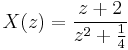
The only zero is located at:  , and the two poles are located at:
  .
.
The pole–zero plot would be:
Interpretation
The region of convergence (ROC) for a given transfer function is a disk or annulus which contains no poles.
- If the disc includes the unit circle, then the system is BIBO stable.
- If the region of convergence extends outward from the largest pole (not at infinity), then the system is right-sided.
- If the region of convergence extends inward from the smallest nonzero pole, then the system is left-sided.
The choice of ROC is not unique, however the ROC is usually chosen to include the unit circle since it is important for most practical systems to have Bounded Input, Bounded Output (BIBO) stability.
See also
Bibliography
- Haag, Michael (June 22, 2005). "Understanding Pole/Zero Plots on the Z-Plane". Connexions. http://cnx.rice.edu/content/m10556/2.8/. Retrieved January 24, 2010.
- Eric W. Weisstein. "Z-Transform". MathWorld. http://mathworld.wolfram.com/Z-Transform.html. Retrieved January 24, 2010.